Demand System Asset Pricing (DSAP) seeks to jointly understand asset prices, macro variables, characteristics, portfolio holdings and flows. In this post, I summarize frequently asked questions and clarify misconceptions associated with recent work in this area. This post is continuously updated.

General Comments

Why now?

1. Availability of higher quality data on institutional and household holdings
2. Structure on demand systems based on factor models and characteristic-based demand
   — Expected return and risk are functions of characteristics
3. New instruments proposed in recent years
4. Many new policy questions are “quantity questions” that can benefit from a well-specified asset demand system.

Comparison to the “SDF Approach”

There is no tension between the “SDF approach” and the “Demand approach.” This is because any asset pricing model that delivers an SDF also delivers a demand system.

Much of the literature has focused on the implications of the model for the cross-section of returns, but not on the implications for the demand system. So instead of testing \(\mathbb{E}[MR]=1\), DSAP seeks to test whether \(Q_i(P)\) is well-specified.
—* Section 5.3 of Gabaix and Koijen (2023) illustrates how to get the SDF once you specified the demand system.*

Another benefit of the demand system is that it also tells you which investors’ demand contributes to the risk price. So even if the SDF is the end goal, the demand system can help.

Demand elasticities in standard models

Asset pricing theories generally imply downward-sloping demand. In other words, if price is higher for whatever reason, people will demand less of it. Typically, this is due to investors being risk averse, hedging demand (adds inelastic component to your demand), or price impact (since you’re trading with people who have superior information to you).

Quantitatively, the demand curves are virtually flat. In the standard CAPM model, idiosyncratic risk is always diversified. So what matters is the stock’s beta and its contribution to aggregate risk. In short, stocks are very close substitutes in the CAPM world.

Residual supply

If someone decides to buy 10% of apple stock, it’s a supply shock of -10% rather than a demand shock of 10%. This is because a given investor \(i\)’s demand is the supply minus the sum of all other investors’ demand. So someone else buying 10% of Apple is like a -10% supply shock to you.

Estimation in levels vs. flows

One can estimate demand from a single cross section on “levels”. However, the same model should also explain “flows” (i.e. in first differences). For example, the index additions/deletions are about flows, and the elasticities from that literature are consistent with the ones estimated on levels (KY 2019, JPE).

Role of Market Clearing

One does not need market clearing to estimate the demand curves. But market clearing is the reason why price is endogenous in the demand estimation and therefore requires an instrument. You also need market clearing to estimate the price impact of a demand shock (and counterfactual equilibrium prices).

Demand elasticity is not a structural parameter

The demand elasticity depends on deep parameters like preferences, number and characteristics of investors, etc. To list a few micro-foundations:

• mean-variance portfolio choice
• portfolio choice with hedging demand (Merton, 1973)
• private information and imperfect competition (Kyle, 1989)
• heterogeneous beliefs
• institutional asset pricing with constraints (Koijen and Yogo, 2023)
• direct preferences for characteristics (e.g. ESG)

However, in Koijen and Yogo (2019) for example, the counterfactual assumes the elasticity is fixed. It then becomes an empirical question whether demand elasticities are sufficiently stable over time and across some types of policxy experiments to make useful predictions.

From Static to Dynamic

There is a “rule of thumb” for converting the one-period price elasticity of demand to a dynamic setting — you can multiply the price elasticity of demand by the dividend yield.

Theory

CAPM generally results in two-fund separation — all investors are predicted to own the same risky asset portfolio. The problem is that in the data, that doesn’t hold both for institutional and individual portfolio holdings data. So you need a model that breaks two-fund separation to match the portfolio holdings data.

Data FAQ

Form 13F

1. Who files 13F? You need to file a 13F if you manage more than $100m worth of stocks, closed-end funds, and ETFs traded on US exchanges. Family offices or rich people usually do not file 13Fs. This is at a quarterly frequency.
2. What can we observe? 13F data are at the level of the institution. So we observe holdings for Vanguard, instead of Vanguard Small Cap Value Index Fund.
3. 13Fs do not provide real-time information. Firms need to file based on their holdings at the end of each calendar quarter, and the filing deadline is 45 days after the end of the quarter.
4. 13Fs do not show swaps or short positions. At the same time, options positions get reported in 13Fs based on the notional value of the position, which makes them open to misinterpretation.
5. Access. 13-F filings can be accessed via Thomson-Reuters (S34; available on WRDS) or FactSet Ownership. There’s also another version called Thomson Reuters Ownership, which is different from the S34. These are public filings so in principle, you can download this from EDGAR. And what Thomson-Reuters does is to organize it for you. The preferred format is to access through FactSet Ownership, which has quality controls that fix errors in the Thomson-Reuters version.
   — FactSet provides correct type codes and identifies hedge funds; there are mistakes in S34 since the late 90s. Authors match on CUSIP (using historical CUSIP) and then aggregate by PERMCO.

Comments on Specific Papers

Koijen-Yogo (JPE 2019)
A Demand System Approach to Asset Pricing

1. If you assume expected returns and factor loadings are linear functions of characteristics, then you get portfolios that are linear in characteristics. If you assume they are polynomial functions of characteristics, you obtain portfolios that are loglinear in characteristics. The latter fits the data better.
   — This is the corollary 1 of the paper. Main idea is that you can expand the set of characteristics with polynomials to approximate the exponential function.
2. The short sale constraint is needed if we want portfolio weights to be positive, as in the 13F data that the authors use.
3. The assumption that \(\beta_0 < 1\) is a sufficient condition for uniqueness of equilibrium. \(\beta_0 > 1\) is economically possible, but for doing counterfactuals it is less convenient as one needs to deal with multiple equilibria.
4. In this paper, you do not need assumptions about the distribution of the error to arrive at logit demand. Remember that there are many ways to arrive at logit demand.
5. \(\beta_0\) in their framework carries the interpretation of the price inelasticity.
6. Standard logit demand structure imposes homogeneous cross-substitution across assets. In a nested logit system, homogeneity is within the nest.
7. The latent demand is modeled as multiplicative to exponential characteristics rather than linearly additive. This allows portfolio weights to be zero when latent demand is zero.
8. When we include investor-quarter fixed effects in the specification, the choice of the outside asset does not matter for estimation since it will get absorbed in the intercept. But the choice of the outside asset will matter in counterfactuals.
9. The addition of zero weights (and using non-linear estimation) matters for the smaller investors where the investment universe really matters.
10. In the counterfactuals, authors take the following approach: 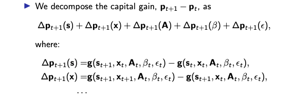Because the functions are non-linear, the order of the decomposition matters. In practice, the outsized role of latent demand is still there.
11. One of the tables shows that large institutions do not account for much variance. Note that this is about the cross-sectional variance across stocks. On the other hand, the evidence from intermediary asset pricing can be considered as a statement about the time-series variation. In reality, large institutions hold close to the market portfolio and therefore there is not much cross-sectional trading.
12. One could presumably add other characteristics like trading volume, turnover, and investor attention. But one needs to be careful as turnover, for instance, depends on latent demand and is therefore also endogenous.

Koijen-Yogo (WP 2020)
Exchange Rates and Asset Prices in a Global Demand System

1. The nested logit specification is not micro-founded in this paper.

Koijen-Richmond-Yogo (RESTUD, 2024)
Which Investors Matter for Equity Valuations and Expected Returns?

1. This paper shows how a standard portfolio choice model implies a linear demand function that depends on prices and characteristics, under the factor assumption.
2. There are a few points of distinction in the estimation procedure when compared to Koijen and Yogo (2019). First, there are more stock characteristics — ESG measures — in the KRY2024. Second, micro caps in KRY2024 are dropped and placed in outside assets to focus on larger firms. Third, authors use ridge which yields more heterogeneity in demand coefficients.

Gabaix-Koijen (JPE 2024)
Granular Instrumental Variables

1. Bartik is very good for the cross-section but not for the aggregate.
2. To have a good precision, we need a high herfindahl (a few large firms, countries, industries, banks), and large idiosyncratic shocks.
3. The GIV allows you to estimate both demand and supply elasticities with one instrument. This seems to be due to the assumption that in this specification: 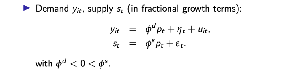\(u_{it}\) enters the first equation with a coefficient of 1, whereas in a typical IV setting the coefficient in front of \(u_{it}\) typically needs to be estimated.
4. The application of GIV extends beyond aggregate elasticity, since an idiosyncratic risk of each individual is a valid shock to all others.
5. In practice, the estimation procedure has both factors and controls. The distinction is useful for cases where you know certain factors are important and you observe them, and you want to use that knowledge and avoid having to estimate them.

Gabaix-Koijen (WP 2022)
In Search of the Origins of Financial Fluctuations: The Inelastic Markets Hypothesis

1. Measuring flows:
2. The elasticity depends critically on whether the demand / supply shocks are anticipated or not. In a dynamic model, prices respond to expected flows and demand shocks. If the actual flow (which was anticipated) then happens, the price impact will be very small. This distinction is also important in this paper by Hartzmark and Solomon (2023).
3. Permanent flows (e.g. you buy a lot today and hold it), you push price up and price stays up. Flip side of this is that E[R] goes down and stays down.
4. In the expression for elasticity, the dividend-price ratio appears: 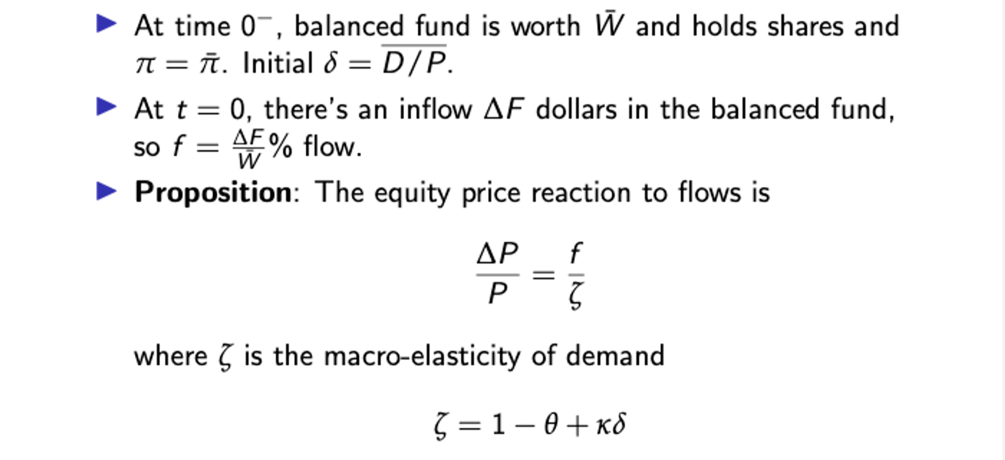The dividend-price ratio appears here because it determines how much expected return falls if you have an exogenous 1% increase in price. And that determines how much one reduces the demand.
   — To see why dividend-price ratio plays this role, expected return depends on two things: D(t+1)/P(t) and P(t+1)/P(t). If the price increase is permanent, the second term remains the same, so only the first term matters)

Useful Links

1. NBER Reporter: Asset Demand Systems in Macro-Finance [link]
2. List of papers using an asset demand system [link]
3. Lecture notes on demand system asset pricing [link]