With the broader availability of panel data, fixed effects (FE) regression models are becoming important and used widely for identifying causal effects. In this post, I discuss a few papers in which the usage of fixed effects is quite illuminating. I have benefited from discussions with Gurpal S. Sran and Jingtao Zheng.

The Basics

In general, one runs into many discussions on what fixed effects (FE) to add and which variation they retain afterwards. Here are some commons from the finance literature:

Source of Concern	Fixed Effect to Add
Unobserved heterogeneity across time (e.g. macroeconomic shocks)	Time FE
Unobserved heterogeneity across individuals (e.g. talent, risk aversion)	Individual FE
Unobserved heterogeneity across industries over time (e.g. investment opportunities, demand shocks)	Industry-Year FE

Some important caveats / tips to keep in mind:

1. FE (without a time subscript) cannot address time-variant unobserved heterogeneity.
   • Often, the fixed effects in Khwaja-Mian (2008) is referred to as adding time-variant fixed effects. These are just firm-year fixed effects.
2. FE restricts analysis to “within” variation. So no-within variation observations do not contribute to the coefficient estimates, which renders the interpretation of the estimate a bit more nuanced.
3. If you have data that has three dimensions you can add three two-way fixed effects. If you have data that has four dimensions, you can add four three-way fixed effects. What this calculation reveals is that it requires a decision on the researcher’s part on which cross-sections to purge and which cross-sections to retain. And naturally, these decisions invite questions regarding external validity.

Example 1. Khwaja and Mian (2009)

I discussed the usage of fixed effects in a separate post earlier. The bottom line is that one can add firm-year-specific effects — if the firm has multiple banking relationships — to control for unobserved credit demand. With enough granularity in data, we can compare the loan growth of a given firm in a given year across two different banks.

Example 2. Hortacsu et al. (2013)

I probed a few of my peers for papers that had the largest dimension of heterogeneity in an empirical setting, and this is what I could find. In this paper, authors examine the effect of firm distress on used cars’ values using the following empirical model:

\[p_{ijklt} = \beta CDS_{it} + X_{ijklt}\Gamma + a_{ijkT} + \epsilon_{ijklt}\]

where the subscripts are:

• \(i\) indexes the car manufacturer
• \(j\) indexes the car model, trim, and model year
• \(k\) indexes auction location
• \(\ell\) indexes the specific auction at which the car is sold
• \(t\) indexes day
• \(T\) indexes week

Therefore, the dependent variable \(p_{ijklt}\) is the transaction price of the car at the auction. The main independent variable \(CDS_{it}\) is the manufacturer credit default swap spread in period \(t\) and \(\beta\) is thus the coefficient of interest. The vector \(X_{ijklt}\) contains other controls describing the car and auction characteristics.

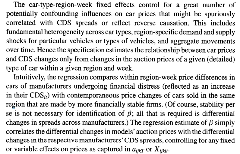
Importantly, \(a_{ijkT}\) is a car type-region-week fixed effect. Notice that the indices not in the fixed effects are \(\ell\) and \(t\). In other words, the effect of firm distress on used cars’ values is being identified off using the variation across auctions and across days within the week for the same car and the same auction location. Here are the authors’ explanation of the same intuition from the paper:

Example 3. Granja (2017)

In this paper, the author studies the effects of reporting and supervisory requirements on financial stability:

\[Y_{ist} = \alpha_{st} + \eta_{it} + \rho_{is} + \beta D_{is,t-1} + \gamma X_{ist} + \epsilon_{ist}\]

where \(Y_{ist}\) is the proportion of ban failures operating in a given state \(s\) in year \(t\) and in the banking system \(i\) and \(D_{is,t-1}\) is an indicator variable that takes the value of 1 if state \(s\) passes state reporting requirements in year \(t-1\) and zero otherwise.

Even before understanding what \(Y\) and \(D\) represent, we can see that this is the maximum level of two-way fixed effect saturation you can do: if you have 3 dimensions of heterogeneity, you can add \(3C2=3\) two-way fixed effects to eliminate not-useful variation. Also, \(X_{ist}\) cannot be a fixed effect, so it must be a control variable.

While the saturation is easy to do, carefully thinking through the economics requires a bit more work:

• State-year FE (\(\alpha_{st}\)): This eliminates the effect of local economic conditions such as a bad crop year or natural disaster.
• Banking System-Year FE (\(\eta_{it}\)): This eliminates the effect of shocks and trends common to a banking system in a given year, most commonly regulatory changes that affect a particular group altogether.
• State-Banking System FE (\(\rho_{is}\)): This eliminates the effect of invariant characteristics of each banking system in each state.

Example 4. Sran (2021)

Gurpal Sran, who is a job market candidate from Booth this year, has a paper which involves examining the correlation between opacity incentives and specificity in job posting for innovation jobs. To provide a little bit more context,

The estimating equation is as follows:

\[Y_{ikct} = \beta FirmOpacity_k + \zeta_{vj} + \lambda_{cj} + \eta_{jdt} + \alpha_{zd} + \epsilon_{ikct}\]

where \(i\) denotes a job posting for an innovation job, \(k\) denotes the employer making the posting, \(c\) denotes the county in which the job is located, \(t\) denotes the year-month of posting, \(d\) denotes the three-digit NAICS code of the employer \(k\), \(j\) denotes the eight-digit ONET code associated with job posting \(i\), \(z\) denotes a decile rank of firm size, and \(v\) denotes the set of job posting features conveyed on job posting \(i\).

Once again, let’s examine the role of the fixed effects:

• County-job Fe \((\lambda_{cj})\): These control for the effect of time-invariant local labor market characteristics of a job posting for job \(j\) hiring in county \(c\).
• Job-Industry-Time FE (\(\eta_{jdt}\)): These control for time-variant factors by job and hiring industry.
• Posting feature-job FE \((\zeta_{vj})\): These control for variation explained by posting features \(v\) for job \(j\)
• Interaction of deciles of firm size and industry \((\alpha_{zd})\): These are included to control for other unobservable firm-level characteristics.

In sum, this design amounts to “comparing postings from two groups of similarly sized firms — one group opaque, the other less so — in the same industry hiring for the same innovation job at the same point in time, after controlling for local labor market characteristics and job posting features.”

The Incidental Parameter Problem

Thus far, we’ve largely abstracted away from major issues involved in fixed effects estimation. Largely, this is because I’ve written the post with a linear model in mind, in which the usage of fixed effects corresponds nicely to taking out the group mean and therefore only looking at the within-group effects.

Using fixed effects in non-linear models, especially those involving maximum likelihood solutions, introduces what’s widely known as the incidental parameter problem. The genesis of the problem starts from the fact that one cannot simply difference the dummy variables and thus the fixed effects need to be estimated along with other parameters of interest as well. (It turns out that for Poisson and logit you can do this.) As a result, the likelihood that needs to be maximized becomes more and more difficult to maximize as parameters that are of minimal interest are introduced incrementally.

Usually this issue pops up when the dependent variable is a binary outcome and one wishes to estimate a probit model. Econometrically, solutions involving the jackknife bais corrections seem to have been proposed, and commands like probitfe and logitfe can be used to correct for the bias.

Useful References

• Ed deHaan (2021), “Using and Interpreting Fixed Effects Models”
• Gormley and Matsa (2014), “Common Errors: How to (and Not to) Control for Unobserved Heterogeneity”
• Fernandez-Val and Weidner (2018), “Fixed Effects Estimation of Large-T Panel Data Models”