In many empirical models within finance, one needs to decide whether to use variables as their levels or their changes. In this post, I briefly go over reasons why one may choose one versus the other.

#1: Perils of Spurious Regressions

The first consideration is the stationarity of the variables in question.

Specifically, one should avoid regressing levels on levels is when \(y_t\) and \(x_t\) are not stationary in the following model:

\[y_t = a + bx_t + e_t\]

where \(y_t = y_{t-1} + v_t\) and \(x_t = x_{t-1} + w_t\) and \(v_t, w_t\) are each IID normal.

In this case, we often have:

• In the limit, the coefficient estimate will follow a non-degenerate distribution
• The t-value is most often significant, and the \(R^2\) is typically very high

Cointegration is one possible way of handling spurious regression, widely used in the macroeconomics literature. In this case, it is safe to run an OLS regression.

• Note: This website contains some fun examples of spurious regressions.

#2: Structure Behind Estimation

The second consideration is the structure that underlies the empirical estimation process. If there is a theory or model that provides guidance, the structure can be informative of whether the level or the change in variable should be included.

As a simple example, suppose one is interested in estimating the Taylor rule:

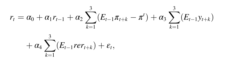
Then you would want to include the level of inflation \((\pi^t)\) rather than the change in inflation \((\Delta \pi^t)\) in the estimation.

#3: Statistical Power

The third consideration pertains to statistical power. This is probably the most important.

Let’s assume both \(y_t\) and \(x_t\) are stationary, and that the true model is given as:

\[y_t = a + bx_t + e_t\]

Furthermore, suppose \(x_t\) and \(e_t\) evolve according to the following processes:

\[x_t = \phi_x x_{t-1} + \xi_t\\ e_t = \phi_e e_{t-1} + u_t\]

Under this setup, we can express the variance of \(x_t\) and \(e_t\) as the following:

\[\sigma^2(x_t) = \frac{\sigma^2(\xi_t)}{1-\phi_x},\quad \sigma^2(e_t) = \frac{\sigma^2(u_t)}{1-\phi_e}\]

Given this setup, we can compute the signal-to-noise ratio when estimating in levels:

\[\frac{\sigma^2(x_t)}{\sigma^2(e_t)} = \frac{\sigma^2(\xi_t)}{\sigma^2(u_t)} \cdot \frac{1-\phi_e}{1-\phi_x}\]

• If \(x_t\) is very persistent with \(\phi_x\) close to 1, but \(e_t\) is IID with \(\phi_e =0\), then this signal-to-noirse ratio is maximized.
• On the other hand, the signal-to-noise ratio from first differencing will much lower since in that case \(\sigma^2(x_t) \gg \sigma^2(\Delta x_t)\).

A simple simulation also confirms this intuition.

• I simulate the above processes assuming \(\xi_t\) and \(u_t\) are i.i.d. normal with mean zero and variance 1. I then vary values of \(\phi_x\) and \(\phi_e\) to see how the signal-to-noise ratios compare.
• As seen below, the signal-to-noise ratio is much higher in the levels specification

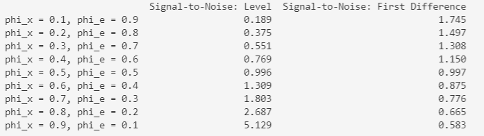
This is also why in the predictive regressions where we regress returns on the dividend-price ratio, it’s important to run it in levels. Estimating the model in first differences will provide very noisy estimates.