Central banks already come equipped with the dual goal of price stability and financial stability. In this post, I explore existing literature that explores the role of financial stability considerations in monetary policy, above and beyond its traditional financial stability tools.

Taylor Rule Galore

Let’s first talk about the Taylor rule and its variants. We will use this framework first to think about what the optimal policy rates should be.

1. Traditional Taylor Rule and Its Variants The traditional Taylor rule is not forward-looking and therefore reacts to contemporary deviations of inflation and output from target. It was introduced by John Taylor in 1993: 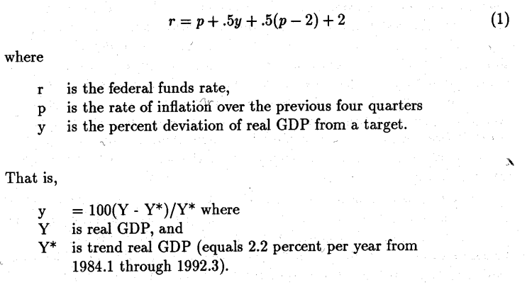The key point in the rule is that the weight on the deviation of inflation from target received a coefficient of 1.5 reflecting the “Taylor Principle” that when inflation rises above target the real interest rate should be increased more than one-for-one. Bernanke offered a modified version of the rule in 2015 by proposing two changes:
   1. Measuring inflation using the core PCE deflator rather than the GDP deflator
   2. Changing the weight on output from \(0.5\) to \(1.0\)
2. Forward-Looking Expectations and Smoothing Clarida, Gali, and Gertler (2000) estimate a forward-looking policy rule for various monetary regimes in the United States. They also allowed for only partial adjustment towards target based on an interest rate smoothing equation: Here are the estimated parameters: 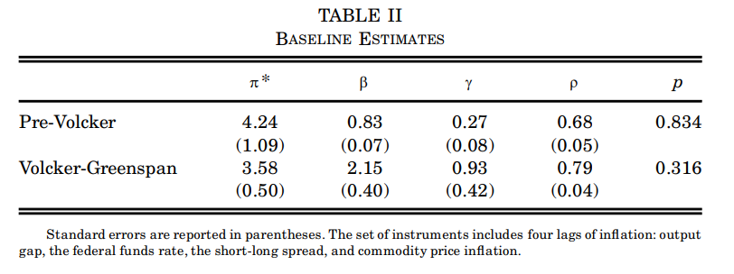So the smoothing parameter is around \(0.8\) and the coefficient on output is \(0.93\). More recently, Clarida explicitly endorsed an alternative policy rule:

   Consistent with our new framework, the relevant policy rule benchmark I will consult after the conditions for liftoff have been met is an inertial Taylor-type rule with a coefficient of zero on the unemployment gap, a coefficient of 1.5 on the gap between core PCE inflation and the 2 percent longer-run goal, and a neutral real policy rate equal to my SEP projection of long-run r*

3. Taylor Rule for Open Economies The baseline Taylor rule might also be inappropriate for open economies subject to external shocks, in which case it may be necessary instead to include other variables such as the ex- change rate.
   • Ball (1999) concluded that such an augmented rule was followed in Canada from 1975 to 2003, whilst Lubik and Schorfheide (2007) found that it was in the UK as well as Canada, but not in Australia and New Zealand. On the other hand, if the exchange rate fluctuations are responded with a different policy instrument, it may not be necessary for exchange rates to appear in the equation determining the policy rate.
   • Daude et al. (2016) pointed out that central banks in emerging markets with a flexible exchange rate regime frequently intervene in their foreign exchange market.
   • Eichengreen and Gupta (2016) also analyze the sudden stops in capital flows to emerging markets since 1991. They argue that the conventional wisdom — that EM central banks tighten monetary and fiscal policies to counter the drop in the exchange rate and in an effort to restore confidence — is evidence in only a minority of cases.
   • Kalemli-Özcan (2019) makes an argument on why domestic monetary policy may be ineffective.

Loss Function for Monetary Policy

Equipped with the Taylor Rule in mind, let us now specify the loss function for a given central bank’s monetary policy. Suppose that the central bank has a target rate based on a standard dual mandate under which it stabilizes the inflation rate around an inflation target and the unemployment rate around its long-run sustainable rate. It also observes a vector of asset prices \(\mathbf{p}_{t}\), *and a vector of asset volatility *\(\boldsymbol{\sigma}_{t}\) in the financial markets.

Following the forward-looking versions of the Taylor rule, the target rate can be expressed as:

\[i_{t}^{*}=\alpha+\beta_{\pi}\left(\mathbb{E}_{t}^{CB}\left[\pi_{t+1}\right]-\pi^{*}\right)+\beta_{y}\left(\mathbb{E}_{t}^{CB}\left[Y_{t+1}\right]-Y^{*}\right)\]

where \(\pi_{t}\) is the inflation rate, \(\pi^{*}\) is the inflation target, \(Y_{t}\) denotes output, and \(Y^{*}\) is the potential output. Importantly, \(\mathbb{E}^{CB}\left[\cdot\right]\) denotes the central bank’s expectations of future inflation and growth.

We then assume that the central bank picks the policy rate \(i_t\) by minimizing the loss function \(L_t\), given by:

\[L_{t}=\left(i_{t}^{*}-i_{t}\right)^{2}+f\left(i_{t};\mathbf{p}_{t},\boldsymbol{\sigma}_{t}\right)\]

where \(f\left(\cdot\right)\) flexibly captures the set of all concerns that the central bank has concerning the asset prices \(\left(\mathbf{p}_{t}\right)\)* *and the volatility \((\boldsymbol{\sigma}_{t})\) in financial market.

The specification therefore implies that the central bank incorporates not only concerns about inflation and unemployment, as reflected in the desire to keep \(i_t^*\) close to \(i_t\), but also direct considerations about the financial markets (represented by \(f\)).

“\(f(\cdot) = 0\)”

In Bernanke and Gertler (1999), asset market fluctuations impact aggregate spending by affecting consumption spending and the cost of external funds via the “financial accelerator” channel. Their main point is that monetary policy should not respond to asset prices beyond its impact on inflation expectations, which became the consensus view and influenced monetary policy during the tech boom.

The Bernanke-Gertler point has been further explored in subsequent work in the context of specific markets:

• Faia and Monacelli (2007) consider a model with credit frictions and show that inflation targeting is preferred to a direct response to asset prices. They use a New Keynesian model with agency costs to argue that responding negatively to asset prices with a Taylor-type interest rate rule is welfare improving.
• Iacoviello (2005) consider a model with credit frictions and show that inflation targeting is preferred to a direct response to asset prices

“\(f(\cdot)\neq0\)”

A large body of work points out, however, that monetary policy should respond to financial conditions above and beyond its effect on output and inflation.

As Kuttner (2011) points out, two implicit assumptions accompany this logic:

1. Financial instability incurs costs other than the volatility in inflation and output, which is outside the scope of Bernanke and Gertler (1999) and its immediate variants.
2. Monetary policy is indeed effective in limiting financial fragility, the exact channel of which depends on the nature of the model in consideration.

Asset Bubbles and Impact of Their Collapse

One line of work focuses on asset bubbles and the economic impact of their collapse.

• Bordo and Jeanne (2002) presents a model in which the collapse of an asset price bubble has repercussions beyond its impact on aggregate demand since it directly impacts the collateral constraints in the productive sector.
• Dupor (2002) presents a theory with irrational firms who over-invest in the presence of an asset price bubble. Monetary policy can therefore be used to respond to these valuation concerns.

Corporate Leverage

Other papers focus specifically on corporate leverage.

• Woodford (2012) presents a model in which \(f\left(i_{t};\mathbf{p}_{t},\boldsymbol{\sigma}_{t}\right)\) is essentially equivalent to welfare losses associated with financial crises, denoted as \(\Omega_{t}\) in his paper, and where the slope of \(f\left(\cdot\right)\) corresponds to \(\lambda_{\Omega}\) in his model. In this model, the welfare loss takes the particular form of distortion of the composition of expenditure between credit-constrained and unconstrained households. The amount of leverage in the economy affects the probability of the occurrence of this welfare loss, and monetary policy can thus act preemptively to prevent this crisis.

Leaning Against the Wind

There is also a growing literature that asks whether central banks should adopt a “leaning against the wind” strategy with respect to asset prices and financial imbalances. Smets (2018) also provides an excellent survey of the trade-offs involved in leaning against the wind policies.

• Svensson (2017) is a recent study that is relatively simple yet very useful for exploring the trade-offs associated with such strategy. He assumes a quadratic loss function of inflation and unemployment with \(f\left(\cdot\right)\neq0\) that represents the cost of a crisis. Through a calibration exercise, he shows that the costs of slowing down the economy are much greater than the gains from reducing risk of a crisis.
• Filardo and Rungcharoenkitkul (2016) and Caballero and Simsek (2019) reach the opposite conclusion with respect to this topic, while Gourio et al. (2018) deliver a more nuanced analysis of when leaning against the wind is worth its costs.

Co-Existence with Macroprudential Policy

A similar debate concerns the potential separation of monetary policy from macroprudential policy.

One view argues that monetary policy should focus exclusively on its traditional mandate while delegating financial stability concerns to macroprudential policy (Svensson (2018)). The other side of the debate highlights the limits of macroprudential policy in dealing with financial excesses (Stein (2014), Gourio et al. (2018)).

Taking\(f(\cdot)\neq0\)as given

There are a few papers that take \(f(\cdot)\neq0\) as given and focus on other aspects of monetary policy.

• Stein and Sunderam (2018) presents a model in which the central bank has private information and is averse to bond market volatility. Therefore, the central bank minimizes \(L_{t}\) where \(f\left(\cdot\right)\) is equal to the volatility of long-term bond yields and \(g\left(\cdot\right)=0.\) Importantly, it takes the market’s conjectures about its behavior as given when minimizing \(L_t\).
• Picault and Raffestin (2020) features a similar loss function and shows that central banks are partially constrained by private market expectations.