Variations in SVARs
In this post, I explore the variations in Structural VARs (SVARs) and their recent applications. This is mostly an amalgam of notes based on my readings of multiple lecture notes, papers, and documentations.
Motivation: Endogeneity Problem in Macroeconomics
Discussion of issues and challenges in identification is as important as in empirical macroeconomics as it is applied microeconomics. Here are two motivating examples:
- Effect of Monetary Policy
- The central bank anticipates a rise in inflation.
- The central bank increases the monetary policy rate, but inflation rises as expected. Conclusion: interest rate hike \(\Rightarrow\) rise in inflation
- Effect of Fiscal Spending
- The government anticipates a decrease in private demand.
- The government increases public spending, but the output decreases nonetheless. Conclusion: public spending \(\Rightarrow\) decline in output
In both examples, the primary issue is that policy choices (rates, fiscal spending) are endogenous to expectations of economic variables (inflation, output). To circumvent this issue, we want to identify purely exogenous shocks.
A Mathematical Formulation
The goal of an SVAR is to go from a reduced form VAR:
\[X_t = F X_{t-1}+e_t\]in which \(e_t\) are not structural shocks, to a structural VAR:
\[AX_t = G X_{t-1} + u_t\]where \(F = A^{-1}G, e_t = A^{-1}u_t\). So as long as we obtain \(A\), we should be done.
How many restrictions are necessary?
The issue is that identifying the \(A\) matrix is not trivial. Let’s start by thinking about how many identification restrictions are necessary for \(A\) to be uniquely identified. Suppose there are \(n\) variables in this specification.
What we do not know: \(n^2\) terms
- The matrix has \(A\) has \(n^2\) unknowns, which can be reduced to \(n^2-n\) by assuming that the diagonals are equal to 1.
- The variance of \(u_t\) has \(n\) terms. (We want structural shocks that are uncorrelated with each other, so the off-diagonals are equal to 0 by assumption)
What we do know: \((n^2 + n)/2\) terms
- The elements in the variance-covariance matrix of \(e_t\), which can be obtained from the estimation. We can obtain the \(n\) diagonals and \((n^2 - n)/2\) off-diagonals. This in total yields \((n^2 + n)/2\).
Above calculation implies that we need \((n^2-n)/2\) additional restrictions to identify the matrix \(A\) (and the structural shocks).
- For 3 variables, we need 3 additional restrictions. For 4 variables, 6 additional restrictions.
Examples of Identification
1. (Zero Short-run) Recursive (Choleski) Identification
This is bascially assuming that the \(A\) matrix is lower triangular.
Stylized Example
\[Y_t = \begin{bmatrix} \pi_t \\y_t\\r_t \end{bmatrix},\quad A = \begin{bmatrix} a_{11} & 0 & 0 \\ a_{21} & a_{22} & 0 \\ a_{31} & a_{32} & a_{33} \\ \end{bmatrix}\]implies that:
- The policy rate \((r_t)\) responds to contemporaneous changes in other variables.
- Output \((y_t)\) responds to current inflation but not current interest rate.
- Inflation \((\pi_t)\) is not contemporaneously affected by policy rate or output. Instead, it only responds to these variables with a lag.
How does this achieve identification?
By setting the upper diagonal elements to zero, we are essentially imposing \((n^2 - n)/2\) additional restrictions. See discussion above on why this is the right number of additional restrictions.
Nota Bene
- Obviously, deciding the ordering (restrictions) to be imposed is crucial. Ideally, we would like to use economic intuition to decide it. Usually, the time frequency of these variables is a consideration.
- The SVAR representation based on recursive identification can be computed using the Choleski factorization of the reduced form covariance matrix — hence its name.
- Let \(A^{-1}\) be the Cholesky factor of \(\Sigma_e\).
- Then since \(e_t = A^{-1}u_t\), we have \(\Sigma_e = \mathbb{E} [A^{-1} u_t u_t' A^{-1'}]\).
- Assuming that \(\Sigma_u = I\), we have \(\Sigma_e = \mathbb{E}[A^{-1}A^{-1'}]\).
Application: Stock and Watson (2001)
- Authors assess the impact of monetary policy \((r_t)\) on unemployment \((u_t)\) and inflation \((\pi_t)\). The size of the VAR is therefore 3.
- The key identifying assumption is that \(r_t\) reacts contemporaneously to movements in \(\pi_t\) and in \(u_t\). Movements in \(r_t\), on the other hand, do not affect contemporaneous \(\pi_t\) or \(u_t\).
2. Zero long-run (Blanchard-Quah) Identification
This identification scheme imposes restrictions on the matrix of the long-run coefficients.
Stylized Example
Consider the VAR model from before: \(X_t = F X_{t-1} + e_t = FX_{t-1} + A^{-1} u_t\). Then the long-run effect of the shock on \(X_t\) is the sum of the short-term effects (impulse responses).
Therefore, the long-run effects can be written as:
\[D=(I+F + F^2 + F^3+\ldots)A^{-1}\]which can be reduced to \(D = (I-F)^{-1}A^{-1}\) if the eigenvalues of \(F\) are in the unit circle.
Now note that \(DD'=(I-F)^{-1}A^{-1}A^{-1'}(I-F)^{-1'}\), but we also know that \(A^{-1}A^{-1'} = \Sigma_e\) that can be estimated. Therefore:
\[DD' = (I-F)^{-1}\Sigma_e (I-F)^{-1'}\]This is where the identification comes in: assume that \(D\) is lower triangular. So only the first shock has a long-run effect on the first variable, and only the first and second shocks have long-run effects on the second variable and so on.
Since \(DD'\) is a symmetric matrix, \(D\) can be obtained using Cholesky decomposition. And once we have that, we can recover \(A^{-1}\) using \(A^{-1} = (I-F)D\) which we can then use to calculate the impulse response functions to the structural shocks.
How does this achieve identification?
This is same as the short-run recursive identification: by setting the upper diagonal elements to zero, we are imposing \((n^2 - n)/2\) additional restrictions.
Nota Bene
- Long-run effect is badly estimated in finite samples. Long-run restrictions transfer this uncertainty to other parameters. (Faust and Leeper (1997))
Application #1: Blanchard and Quah (1989)
- Authors asess the impact of demand and supply shocks on output and unemployment. The size of the VAR is therefore 2.
- The key identifying assumption is that demand-side shocks have no “long-run” effect on the level of output, while supply-side shocks do.
Application #2: Galí (1999)
- Author assesses the impact of technology shock
- The key identifying assumption is that only technology innovations can affect labor productivity in the long-run. As discussed in Gali (1999), this assumption holds in a broad class of models under relatively weak assumptions about the form of the production function.
3. Sign Restrictions
There are multiple ways to decompose the variance of \(\Sigma_e = P'P\).
- Cholesky is unique because it imposes the restriction that \(P\) be lower triangular.
To pin down a unique value of \(P\), we check whether the impulse responses implied by \(P\) satisfy a set of sign restrictions, typically in a theory-driven way.
Stylized Example
According to conventional wisdom, a contractionary monetary policy should:
- Raise the federal fund rate
- Lower prices
We are interested in how it affects output, so we leave output unrestricted. Then we keep only the matrices which generate the responses to a monetary policy shock coherent with 1. and 2.
Nota Bene
- Steps to implement sign restrictions are as follows:
- Estimate the reduced form VAR and obtain \(F\) and \(\Sigma_e\).
- Compute \(P = chol(\Sigma_e)\).
- Draw a random orthonormal matrix \(S\) and compute \(A^{-1} = P'S'\).
- Compute the impulse responses associated with \(A^{-1}\).
- Are the sign restrictions satisfied?
- If yes, store the impulse response.
- If no, discard the impulse response.
- Repeat 3 — 5 until you obtain \(N\) replications.
- Report the mean or median impulse response (and its confidence interval)
Application: Uhlig (2005)
- Author assesses the impact of monetary policy on real GDP. The VAR is of dimension 6: real GDP, real GDP deflator, a commodity price index, total reserves, non-borrowed reserves, and the federal funds rate.
- The key identifying assumption is the set of conventional wisdoms: monetary contractions should raise the federal funds rate, lower prices, and decrease non-borrowed reserves.
4. Narrative Sign Restrictions
This approach constrains the structural shocks and/or the historical decomposition around key historical events, ensuring that they agree with the established narrative account of these episodes.
Stylized Example: Antolin-Diaz and Rubio-Ramirez (2018)
Consider a VAR with three variables: (1) growth rate of global oil production, (2) index of real economic activity, and (3) log of the real price of oil.
A traditional sign restrictions looks something like the following:
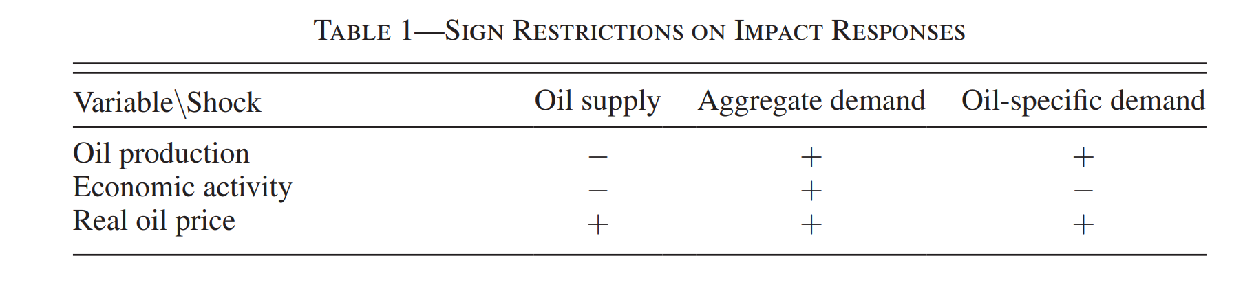
On the other hand, narrative sign restrictions look like the following:
- The oil supply shock must take negative values in December 1978–January 1979, September–October 1980, August 1990, December 2002, March 2003 and February 2011.
- For above periods, the absolute value of the contribution of oil supply shocks is larger than the absolute value of the contribution of any other structural shock.
The implementation steps are otherwise similar as described above.
Nota Bene
5. External Instruments (Proxy SVAR)
This approach uses an external instrument that is correlated with the target shock (the instrument is relevant) but uncorrelated with other shocks of the model (the instrument is exogenous).
Stylized Example
Consider a VAR with two variables — \(r_t\) and \(y_t\) — that takes the following standard form:
\[\begin{bmatrix}y_t \\ r_t \end{bmatrix} = \begin{bmatrix} \phi_{11} & \phi_{12} \\ \phi_{21} & \phi_{22}\end{bmatrix} \begin{bmatrix}y_{t-1} \\ r_{t-1} \end{bmatrix} + \begin{bmatrix} a_{11} & a_{12} \\ a_{21} & a_{22}\end{bmatrix}\begin{bmatrix}u_t^1 \\ u_t^2 \end{bmatrix}\]Suppose we are interested in identifying \(u_t^1\) and that we have a valid external instrument \(z_t\) that satisfies \(\mathbb{E}[z_t u_t^1]\neq 0\) and \(\mathbb{E}[z_t u_t^2] =0\).
Recall that we have:
\[e_t^1 = a_{11} u_t^1 + a_{12}u_t^2\\ e_t^2 = a_{21}u_t^1 + a_{22}u_t^2\]- Estimate the reduced form system to obain estimates of the reduced form residuals, \(e_t\).
- Estimate the following regression: \(e_t^2 = \beta z_t + \xi_t\) in which case \(\hat{\beta} = Cov(e_t^2, z_t) / Var(z_t)\) By our identifying assumption, \(Cov(e_t^2,z_t) = a_{22} Cov(u_t^2, z_t)\).
- Estimate the following regression: \(e_t^1 = \gamma \hat{e}_t^2 + \zeta_t = \gamma \hat{\beta}z_t + \zeta_t\) in which case \(\gamma \hat{\beta} = Cov(e_t^1, z_t) / Var(z_t)\) By our identifying assumption, \(Cov(e_t^1, z_t) = a_{12} Cov(u_t^2, z_t)\).
- Combining steps 2 & 3, we have \(\gamma = a_{12} / a_{22}\).
Finally, we can normalize \(a_{22}\) to be equal to 1, in which case \(a_{12} = \gamma\).
Nota Bene
Application: Gertler and Karadi (2015)
  - Authors assess the impact of monetary policy on real GDP. The VAR is of dimension 4: industrial production, the consumer price index, the 1-year T-bill interest rate, and the excess bond premium.
  - The key identifying assumption is that there exists an external instrument such that (1) it is correlated with the monetary policy shock and (2) it is uncorrelated with all other structural shocks in the system.
     - In this paper, such external instrument is the high-frequency monetary surprise measured using a 30-minute window around FOMC announcements.
What can you do with SVARs?
1. Impulse Response
The impulse response function traces the effect of a one-time shock to one of the structural errors on the current and future values of all the endogenous variables, assuming that the other structural shocks are kept to zero.
- Example: What is the impact of a monetary policy shock to GDP?
This is only possible when the errors are uncorrelated, hence the emphasis on uncovering the “structural” model.
- The impulse responses are easy to compute: \(IRF(0) = A^{-1}, IRF(1) = FA^{-1}, ...\)
2. (Forecast Error) Variance Decomposition
The variance decomposition separates the variation in a endogenous variable (forecaste rrors) into the component shocks of the VAR. It provides information about the relative importance of each innovation in affecting the variables.
- Example: What is the (average) importance of demand shocks in driving GDP forecast errors?
The forecast error at horizon \(t-h\) is with respect to \(t-1\):
\[FE_{t+h} = X_{t+h} - \mathbb{E}[X_{t+h}] = \sum_{i=0}^h F^{h-i} A^{-1}u_t\]To decompose the variance, it helps that each component of \(u_t\) are orthogonal to each other. Therefore, the variance decomposition can be obtained from the squared magnitudes of the individual elements in \(F^{h-i}\).
3. Historical Decomposition
Historical decomposition separates the historical contribution of each structural shock in driving deviations of the VAR’s the endogenous variables away from their equilibrium.
- Example: What was the contribution of oil shocks in driving the fall in GDP growth in 1973:Q4?
The key is to write \(X_t\) as a function of present and past structual shocks. For simplicity, let’s consider \(t=2\):
\[X_2 = F^2 X_0 +FA^{-1}u_1+A^{-2}u_2\]Python Implementation
For Matlab, I suggest using this toolbox by Ambrogio Cesa-Bianchi.
For Python, a basic VAR can be implemented using statsmodels:
import pandas as pd
import numpy as np
import statsmodels.api as sm
from statsmodels.tsa.api import VAR
The libraries for more advanced VARs with restrictions do not seem readily available in Python. One alternative is to use packages from R.